Database Internals Ch. 2 - B-Tree Basics

Database Internals - Ch. 2 - B-Tree Basics

8 minute read • February 2, 2026

This post contains my notes on Chapter 2 of Database Internals by Alex Petrov. The chapter introduces us to the B-Tree data structure and explains why and how database engines use them. These notes are intended as a reference and are not meant as a substitute for the original text. I found Timilehin Adeniran’s notes on Designing Data-Intensive Applications extremely helpful while reading that book, so I thought I’d try to do the same here.

Binary Search Trees

Binary Search Trees (BSTs) are sorted, in-memory data structures used for efficient key-value lookups. Each node possibly points to left and right nodes, with each being considered a “subtree”. All nodes to the left of a given node have values less than the node’s values, and all nodes to the right have greater values. This allows us to use the Binary Search algorithm to find the target node in O(logN) time, where N is the number of nodes. Every time a node is compared to the target value, we are able to discard half of the search space (assuming the tree is balanced).

Tree Balancing

Standard BSTs do not specify a pattern for inserting data, which can sometimes lead to “unbalanced” trees. In the worst case, our tree ends up looking like a linked list, and searches could take O(N) comparisons instead of O(logN).

We consider a tree to be balanced if its height is minimized to logN and the difference in height between any two of its subtrees never exceeds 1. This ensures logarithmic lookup complexity. Balancing operations such as pivots and rotations are performed after some or all updates and deletions, depending on the specific data structure. We define fanout as the maximum number of children per node. Fanout and height are inversely correlated.

Trees for Disk-Based Storage

There are several problems with using BSTs on disk-based storage:

locality - there is no guarantee that child nodes are near their parent on disk, requiring more disk seeks, which are especially costly on HDDs. This is mitigated by “Paged” Binary Trees.
tree height - since Binary Tree fanout is low (2), we have to perform up to logN seeks to find data

The most suitable tree for on-disk storage should therefore have:

high fanout to improve locality of neighboring keys
low height to reduce the number of seeks during traversal

Disk-Based Structures

See my notes on chapter 1 for a brief description of Memory-Based vs. Disk-Based DBMS.

Hard Disk Drives (HDDs)

Most algorithms were developed when spinning disks were still the most common form of storage. On spinning disks, seeks increase the costs of random reads because they require disk rotations to physically move the read/write head. However, reading and writing contiguous data is relatively cheap. This is why locality is so important.

Solid State Drives (SSDs)

On SSDs there are no moving parts. They consist of memory cells. The hierarchy of memory on SSDs is as follows: memory cells > strings > arrays > pages > blocks > planes > dies.

The smallest chunk that can be written is the page, but only empty memory cells on the page. The smallest size that can be erased is a block of pages called an “erase block”. Pages in empty blocks have to be written sequentially.

The Flash Translation Layer (FTL) is responsible for mapping page IDs to physical locations, garbage collection (GC), and for moving and remapping pages. Garbage collection can hurt performance, but it can be mitigated by buffering and immutability.

Compared to HDDs, SSDs don’t require as much attention paid to sequential vs. random IO. Block device abstractions are used by OSs to hide internal disk structures and handle the addressing of chunks of memory, abstracting away some of the physical details.

On-Disk Structures

On-disk structures are designed with their target storage specifics in mind, and generally opt for fewer disk addresses. This can be achieved by improving locality, opting for internal representations of data structures, and reducing the number of out-of-page pointers. This is mostly achieved via high fanout and low height, which are key characteristics of B-Trees.

Ubiquitous B-Trees

Like BSTs, B-Trees are sorted data structures that support efficient searching. B-Trees are efficient for both point queries (finding an exact value) and range queries (finding all values less than a value, greater than a value, etc.).

Note

Most of the examples in this book use a sub-category of B-Trees called B⁺-Trees.

B-Tree Hierarchy

B-Trees consist of nodes, each storing up to N keys and N+1 pointers to children (where N defines the capacity). There are three main types of nodes: the root node, internal nodes, and leaf nodes, which hold the actual key-value pairs. We define occupancy as the node’s capacity vs. the number of keys the node actually holds.

High fanout amortizes the cost of balancing operations which are triggered when nodes “overflow” and become too full or “underflow” and are nearly empty. Many implementations also add pointers between siblings to make range query traversals more efficient.

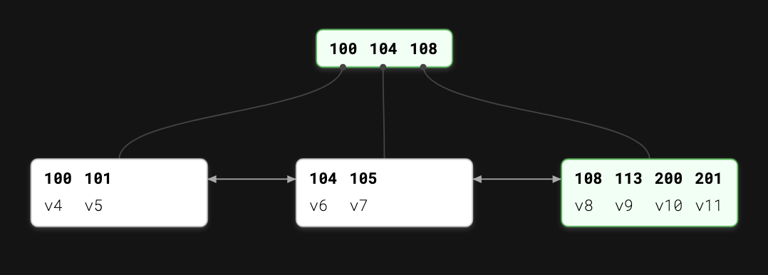
Separator Keys

Separator keys, also called “index entries”, or “divider cells”, split the tree into subtrees, holding corresponding key ranges. Keys are stored in sorted order. The first key points to a subtree where all values are less than the key’s values. The last key points to a subtree where all values are greater. Intermediate keys point to subtrees where all values fit in the range between itself and the next key.

An example of a B-Tree

B-Tree Lookup Complexity

During lookups, at most log_NM pages are addressed, where N is the number of keys in a node and M is the number of items in the tree. At most logM comparisons occur, since Binary Search is used to search across the keys in current node.

B-Tree Lookup Algorithm

Starting from the root, we perform Binary Search on its keys until a separator key is found that is greater than the searched value, giving us a subtree where we can repeat the process. For point queries, the search is done after finding (or not finding) the searched key in the leaf nodes. For range queries, iteration starts from the closest found key and follows siblings until the end of the range is reached or no more matching nodes are found.

B-Tree Node Splits

To insert a node, we first have to locate the target leaf and find an insert point using the above algorithm. If the target node has overflowed it must be split in two. A node is split if it is a leaf node already at capacity for key-value pairs, or if it is an internal node already at capacity for pointers.

Splits are done by allocating a new node, transferring half of the elements in the existing node to the new node, and then adding its first key and pointer to the parent node (the key is “promoted”). If the parent node is full, it must be split again. This process propagates up the tree until the parent is no longer full. If the entire tree is full, a new root is created, the existing root is split and demoted, and the height grows by 1.

B-Tree Node Merges

Deletion starts by locating the target leaf, finding the key-value pair, and then removing it. If the occupancy of neighboring nodes falls below a threshold (“underflows”), siblings are merged. Neighboring nodes are merged if they are leaves and the combined total of key-value pairs is ≤N, or if they are internal nodes and the combined total of pointers is ≤N+1. Like with splits, merges can recursively propagate up the tree all the way to the root.

Note

One technique for reducing the number of splits and merges is “rebalancing”

Other Resources

Ben Dicken of PlanetScale has a deep dive on B-Trees in the context of databases called B-trees and database indexes. He also has a YouTube video covering this material. The channel Spanning Tree also has an excellent video on the data structure.

Ben also provided a great web app for visualizing B-Trees.

< All Articles